Options and the Black–Scholes Formula (Part 2)

Part 2

In Part 1 we discussed the difficulties of the equation we obtained:

1. We don’t know anything about the drift parameter μ(t). Intuitively, this is a “risk” parameter for a particular stock/coin/token (but formally the risk parameter is defined differently; a formula will appear below). And this parameter may depend on time.
2. The current equation is quite hard to solve. We can’t just integrate it, because the right-hand side contains non-constant coefficients μ(t)S and σS.

Let’s solve the problems one by one

DISCLAIMER: in these articles I’m trying to give intuition for what’s going on, so in many places I intentionally omit mathematical formalities in order not to make understanding harder.

Let’s take a short detour and recall how the value of a risk-free asset is usually defined.

A risk-free asset is, for example, bonds. That is, instruments that guarantee future income at a rate r, called the risk-free interest rate. For example, such instruments are used to protect against inflation.

For simplicity, let’s assume the risk-free interest rate is constant.

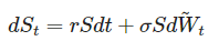
Then the differential equation for the value of a risk-free asset (a bond) is given by:

A bond has no stochastic component, and its drift equals r, which is known to everyone (for example, r = 0.1 means the risk-free rate is 10% per year).

The equation for the price of a risky asset was defined as:

Let’s imagine what would happen if our parameter μ were not an arbitrary function, but, for example, the risk-free rate r.

That is, if our equation looked like this:

Then we would have one fewer unknown and we could already try to solve this equation.

In general, it would be great to get rid of the unknown drift. But can we do that somehow?

It turns out, yes!

Girsanov’s theorem allows us to do this.

If you recall mathematical analysis (and omit the additional conditions of the theorem), there is a theorem that allows moving between measures (the Radon–Nikodym theorem), and the “transition coefficient” between measures is the Radon–Nikodym derivative:

ν, λ are Lebesgue measures.

In our case, the Radon–Nikodym derivative will no longer be a real-valued function, but a stochastic process.

Girsanov’s theorem and the risk-neutral measure

In essence, from the equation

we want to obtain

At first glance it seems impossible. It turns out we just need to move to another probability measure — the “risk-neutral” one.

First, let me remind you what a martingale is.

A martingale is a random process in which the best prediction of the future value is the current value.

We have an equation under measure P:

But Sₜ is not a martingale under measure P, because there is a drift μ(t)Sₜ ≠ 0.

Recall that the equation for the bond price is:

Our goal

Find a measure Q such that the parameter μ does not appear in it at all.

Let’s consider the discounted price of the underlying asset under measure P: {Sₜ / Bₜ}.

Such a process is not a martingale under measure P. But if we make this process a martingale, then we will see that under measure Q we will get rid of the unknown drift μ.

Let’s write a differential equation for this process. Applying Itô’s lemma to it, we obtain:

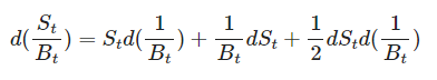
Substituting the equations for dSₜ and dBₜ:

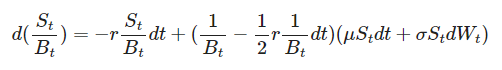
Simplifying this expression and discarding terms of order higher than dt, we obtain the final formula for the process {Sₜ / Bₜ}:

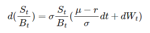
And now the most important part

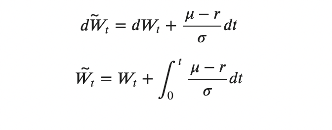
Notice that if we make the substitution:

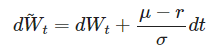
then the process

will be a martingale.

Now let’s see what the process Sₜ looks like under such a change of measure.

We express dWₜ through dŴₜ and substitute into the equation for dSₜ:

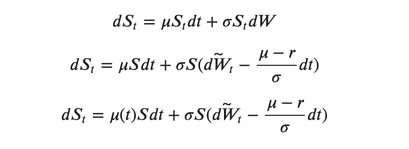
Finally, we get:

dŴₜ is a Wiener process under measure Q.

Why is dŴₜ a Wiener process under measure Q?

Girsanov’s theorem answers this.

Let there be a process {αₜ}ₜ∈[0,T], adapted to the filtration generated by the Wiener process {Wₜ}ₜ∈[0,T] (under measure P).

Define the “stochastic exponential”:

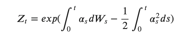
If Zₜ is a positive martingale and Eᴾ[Zₜ] = 1, then Zₜ is the Radon–Nikodym derivative for moving to measure Q,

and the process

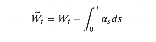
is Wiener under measure Q.

That is

We made the following change of measure:

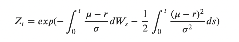
So, in our case:

This means that the process Zₜ is defined as follows:

It’s easy to check that the process Zₜ is indeed a positive martingale and satisfies Eᴾ[Zₜ] = 1:

1. Consider Eᴾ[Zₜ] as a product of expectations of exponentials.
2. Note that one factor is the expectation of a log-normal random variable, and then everything cancels.

And that means the process

is indeed a Wiener process under measure Q.

Thus, we moved to a probability measure where the unknown parameter μ becomes equal to the interest rate r. Moreover, we initially considered the discounted price Sₜ/Bₜ under a measure in which the discounted price is a martingale. That’s why this measure is also called a martingale measure.

P.S. the price must be discounted.

So, we solved Problem 1.

We found a measure in which the drift turns from the unknown function μ into the risk-free interest rate r.

Problem 2 remains.

Now that there is no unknown function μ(t), we can solve the resulting equation:

Such a process is called geometric Brownian motion with constant drift.

How to solve this equation and derive the Black–Scholes equation, I’ll explain in the next article.

Thanks for your time.

Follow the updates.