Introduction

Volatility is one of the most important parameters in option pricing, risk management, and building trading strategies. The classical Black–Scholes–Merton model, which assumes constant volatility, cannot reflect real market dynamics, where “volatility smile” and clustering effects are observed. To describe market processes more accurately, stochastic volatility models were developed; the most well-known among them are the Heston model and the SABR model. These approaches take into account the random nature of volatility changes and allow derivatives to be valued more adequately.

The “Volatility Smile” and Its Impact on Models

Since the financial market crash of 1987, it has been observed that the volatility of options with lower underlying prices is higher than that of options with higher underlying prices. This indicates the stochastic nature of volatility, which varies over time and depending on the underlying price level. Economists developed stochastic volatility models to account for this effect.

The volatility smile (volatility smile) is a graphical representation of the dependence of implied volatility on strike for options with the same time to expiration. Typically, implied volatility tends to increase for both deep in-the-money and deep out-of-the-money options, creating a shape resembling a smile.

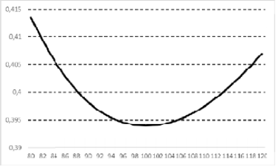
Volatility smile chart

Mathematically, the volatility smile is defined as a function of implied volatility from strike for a fixed time to expiration :

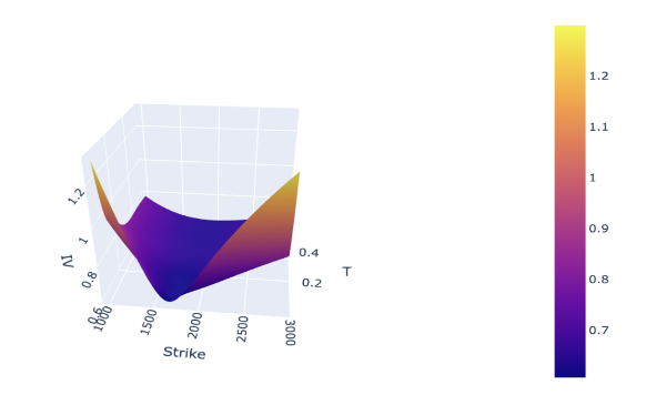
A volatility surface (volatility surface) is a three-dimensional representation of volatility, showing how implied volatility changes depending on strike and time to option expiration. The volatility surface helps to better understand and model market expectations about future fluctuations of the underlying price.

Mathematically, the volatility surface is defined as a function of strike and time to expiration :

This surface is used to determine implied volatility for various strikes and expirations, which is a key element in option pricing and risk management.

Visually, a volatility surface is a plot where:

• X-axis — strike,

• Y-axis — time to expiration,

• Z-axis — implied volatility.

An example of a volatility surface can be built using market option prices and then interpolated or extrapolated to obtain a continuous surface.

Example of a volatility surface

The “volatility smile” reflects the fact that the implied volatility of options with different strikes differs, even though their expiration and underlying are the same. Graphically, it appears as a parabolic shape with edges bent upward.

This phenomenon contradicts the Black–Scholes model, which assumes volatility should be the same for all strikes. Reality showed that after the 1987 crash, traders recognized the possibility of extreme events and price distortions, which required revisiting volatility models.

An alternative explanation of the volatility smile: a market maker, selling options near at-the-money, hedges with more out-of-the-money options; other players who sold those OTM options hedge with even farther ones, and so on. Thus, open positions are distributed step-by-step across the volatility surface.

The Problem of Changing Volatility

In real markets, volatility changes under the influence of many factors: macroeconomic news, liquidity changes, psychological behavior of market participants, and others. Two key properties of volatility that should be taken into account:

• Mean reversion: after sharp spikes, volatility tends to return to its long-term average.
• Volatility clustering: periods of high volatility are often followed by phases of relative calm, indicating time correlation.

Ignoring these features can lead to incorrect option valuations, hedging errors, and mistakes in arbitrage strategies.

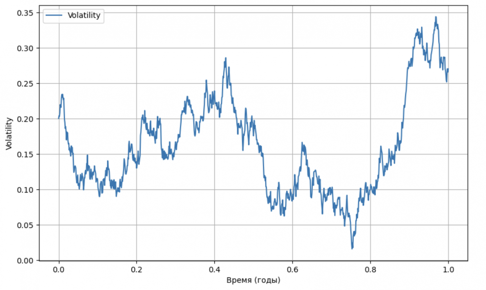
“Mean reversion” of volatility, simulation from the Heston model

The Heston Model

In 1993, Steven Heston, in his paper “A Closed-Form Solution for Options with Stochastic Volatility with Applications to Bond and Currency Options” \cite{heston1993closed}, proposed his model for pricing derivatives. The main idea is to model stochastic volatility with mean reversion.

Approximately this behavior is observed in real markets: for a long time volatility fluctuates around a mean value, in rare cases it “explodes,” and after some time returns to the mean. The model is described by the following system of stochastic differential equations:

where:

• — the underlying price at time t;
• — instantaneous variance (volatility squared);
• — average asset return;
• — speed of mean reversion of volatility to the long-run mean ;
• — volatility of volatility (“vol-of-vol”);

Correlation between the Brownian motions and is described as:

What are the advantages of the Heston model?

Unlike the Black–Scholes model, where volatility is fixed, the Heston model accounts for its random fluctuations over time, which makes it more realistic. Volatility does not remain high or low forever but tends toward a certain long-term mean value, which matches real market behavior.

An important advantage of the Heston model is that for European call and put options there is an analytical solution within this model. This makes it possible to perform fast, computationally inexpensive calibration of the volatility surface for European options.

Are there any disadvantages?

One of the main issues with the model is high computational complexity. Despite the fact that for some cases (for example, European options) analytical solutions can be obtained, in a number of cases one has to resort to numerical methods such as Fourier-integration methods or Monte Carlo simulation. This not only slows down derivative valuation but also complicates model parameter calibration.

In practice, calibration is often carried out using optimization algorithms such as Levenberg–Marquardt, which significantly speeds up the calibration process.

In order for variance to remain strictly positive, the so-called Feller condition must hold:

In practice, however, it often turns out that this balance is violated, especially when calibrating the model on data with a high level of volatility. Violation of the Feller condition can lead to the appearance of small negative volatility values in numerical simulations, which creates additional difficulties in interpreting results and requires special correction methods.

The SABR Model

The SABR model (Stochastic Alpha, Beta, Rho) was first introduced by Patrick Hagan, Andrew Lesniewski, and Diana Woodward in 2002 in the paper “Managing Smile Risk”. The dynamics of the model are described as follows:

This model is described by the following stochastic differential equations:

Parameter constraints: , ,

where:

• — the forward price at time ,
• — asset volatility at time ,
• — the “volatility of volatility” parameter,
• — a parameter that determines the degree of dependence of volatility on the asset price.

Similar to the Heston model, the correlation between the Brownian motions and is defined as:

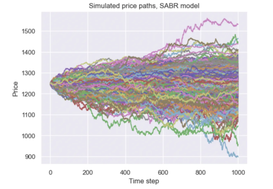
Calibrating the SABR Model

For convenience, let’s introduce new notation:

Then the formula for implied volatility becomes:

Our task is to find partial derivatives of with respect to parameters

Next, we use the Levenberg–Marquardt algorithm for calibration.

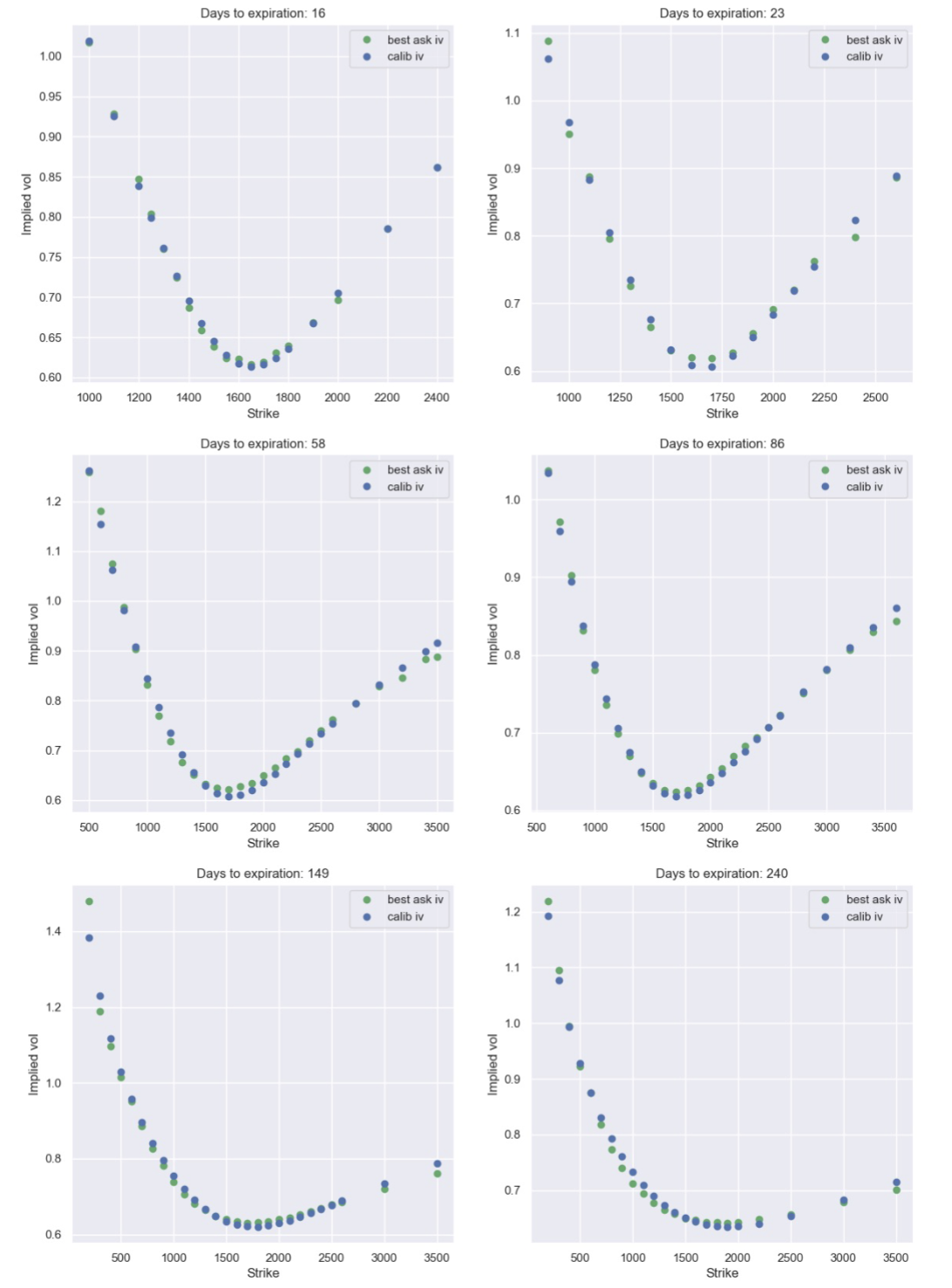
Calibration results of the SABR model applied to Ethereum options on Deribit

Studies show that on the crypto-options market, the SABR model often demonstrates higher accuracy, especially for options with short expirations, while the Heston model can have larger error under imperfect calibration.

Advantages of the SABR model:

One of the key strengths of the model is the availability of approximate formulas for calculating implied volatility. These formulas allow option premia to be estimated fairly quickly, which is especially important when working with large data volumes or in situations where fast decisions are needed.

In addition, the SABR model can reproduce the observed market volatility smile quite accurately. Thanks to the parameter the model adapts to different types of underlying dynamics: at it approaches a log-normal distribution, and at — a normal one. Such flexibility allows the model to be used for a wide range of financial instruments, from interest rates to FX derivatives.

What limitations might there be?

We know that the parameter has a significant impact on the shape of the underlying distribution. An incorrect estimate or choice can distort results. In addition, the optimal value of may vary across asset classes or even change over time, requiring extra attention during calibration.

It is important to consider that the SABR model may require adjustments or extensions to reflect real market processes more accurately, especially when working with exotic instruments or under high instability.

Practical Applications

Stochastic volatility models are used in the following areas:

• Market making: accurate models help set optimal quotes, reducing the risk of losses due to sharp market moves.
• Risk management: models are used to forecast extreme events and adjust portfolios under high volatility.
• Algorithmic trading: fast assessment of short-term volatility changes makes it possible to take quick decisions in high-frequency strategies.

Applying these models contributes to more accurate derivative valuation and reduced operational risks.

Conclusion

Stochastic volatility models such as Heston and SABR significantly expand the capabilities of classical approaches to option pricing. The Heston model provides deep insight into volatility dynamics with mean reversion, but requires significant computational resources. The SABR model, thanks to analytic approximations and simpler calibration, shows high accuracy, especially for short-term valuation.

Choosing the right model and tuning it properly makes it possible to reflect market processes adequately, which is critical for risk management and for building effective trading strategies.

We’ll talk about how to calibrate the entire volatility surface in the next articles.

Thank you for your time!

Notes

• Heston model (Wikipedia)
• Managing Smile Risk